40 excel pivot chart rotate axis labels
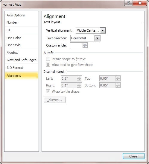
How to rotate text in axis category labels of Pivot Chart in Excel 2007? Select your chart Choose Layout > Axis Titles > Primary Vertical Axis > Horizontal Title or Select your Vertical Axis Title Right click and choose Format Axis Title Select Alignment and you can change both Text Direction and Custom Angle. Both work in Excel 2010 (I don't have Excel 2007 to test, but they should be about the same). Join LiveJournal Password requirements: 6 to 30 characters long; ASCII characters only (characters found on a standard US keyboard); must contain at least 4 different symbols;
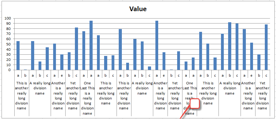
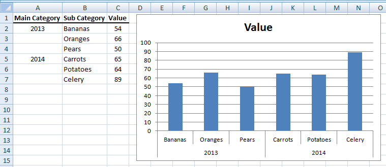
How to group (two-level) axis labels in a chart in Excel? - ExtendOffice The Pivot Chart tool is so powerful that it can help you to create a chart with one kind of labels grouped by another kind of labels in a two-lever axis easily in Excel. You can do as follows: 1. Create a Pivot Chart with selecting the source data, and: (1) In Excel 2007 and 2010, clicking the PivotTable > PivotChart in the Tables group on the ...

Excel pivot chart rotate axis labels
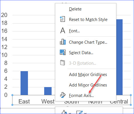
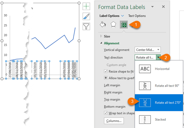
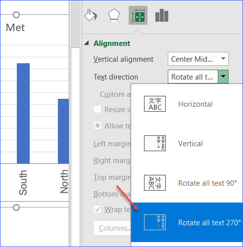
How to rotate axis labels in chart in Excel? - ExtendOffice Go to the chart and right click its axis labels you will rotate, and select the Format Axis from the context menu. 2. In the Format Axis pane in the right, click the Size & Properties button, click the Text direction box, and specify one direction from the drop down list. See screen shot below: The Best Office Productivity Tools How to Show Percentage in Pie Chart in Excel? - GeeksforGeeks Jun 29, 2021 · The steps are as follows : Insert the data set in the form of a table as shown above in the cells of the Excel sheet. Select the data set and go to the Insert tab at the top of the Excel window.; Now, select Insert Doughnut or Pie chart.A drop-down will appear. Rotating axis text in pivot charts. | MrExcel Message Board Right Click on the Axis and choose Format Axis. Then find the Alignment area (depends on your version) Then Change Text Direction to Rotate All Text 270 degrees. Note that this will work only on the top level if you are utilizing the "Multi-Level Category Labels" feature of the chart. (i.e. if you have a grouped axis) Steve=True S Surveza
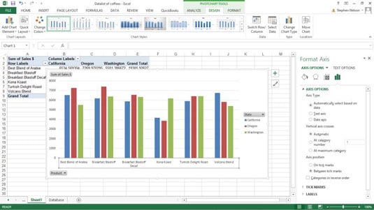
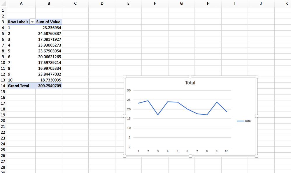
Excel pivot chart rotate axis labels. › make-a-pareto-chart-usingHow to Make a Pareto Chart Using Pivot Tables in Excel Jul 18, 2022 · A useful guide to make a Pareto chart using Excel Pivot Tables. Download our practice book, modify data and exercise. Pivot Chart Horizontal axis will not let me change both Axis categories ... 1. Click the horizontal axis, click the Axis Options button on the Format Axis pane. 2. Select Labels, clear the checkbox of Multi-level Category Labels: 3. Click the Size & Properties button, change the Text direction to Vertical and check the result: Hope you can find this helpful. Best regards, Yuki Sun. - Automate Excel Mar 07, 2022 · Chart Axis Text Instead of Numbers: Copy Chart Format: Create Chart with Date or Time: Curve Fitting: Export Chart as PDF: Add Axis Labels: Add Secondary Axis: Change Chart Series Name: Change Horizontal Axis Values: Create Chart in a Cell: Graph an Equation or Function: Overlay Two Graphs: Plot Multiple Lines: Rotate Pie Chart: Switch X and Y ... › excel-charts-title-axis-legendExcel charts: add title, customize chart axis, legend and ... Oct 29, 2015 · For most chart types, the vertical axis (aka value or Y axis) and horizontal axis (aka category or X axis) are added automatically when you make a chart in Excel. You can show or hide chart axes by clicking the Chart Elements button , then clicking the arrow next to Axes , and then checking the boxes for the axes you want to show and unchecking ...
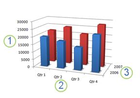
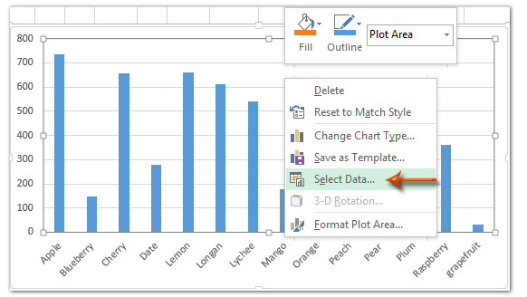
Excel - Quick Guide - tutorialspoint.com You can change the X axis of the chart by giving different inputs to X-axis of chart. You can change the Y axis of chart by giving different inputs to Y-axis of chart. Pivot Charts Excel 2010 Pivot Charts. A pivot chart is a graphical representation of a data summary, displayed in a pivot table. A pivot chart is always based on a pivot table. Change axis labels in a chart - support.microsoft.com Right-click the category labels you want to change, and click Select Data. In the Horizontal (Category) Axis Labels box, click Edit. In the Axis label range box, enter the labels you want to use, separated by commas. For example, type Quarter 1,Quarter 2,Quarter 3,Quarter 4. Change the format of text and numbers in labels Make SECOND x axis rotate on pivot chart | MrExcel Message Board I've made a pivot chart (simple line chart) in Excel 2007 that has two X axis categories (i.e. two fields in the row labels section). Since the X axis labels are quite cluttered I want them BOTH rotated to read vertically, but it seems I can only rotate the one axis? Anyone know if there is a hack to fix this? Many thanks Excel Facts › documents › excelHow to group (two-level) axis labels in a chart in Excel? The Pivot Chart tool is so powerful that it can help you to create a chart with one kind of labels grouped by another kind of labels in a two-lever axis easily in Excel. You can do as follows: 1. Create a Pivot Chart with selecting the source data, and: (1) In Excel 2007 and 2010, clicking the PivotTable > PivotChart in the Tables group on the ...
Rotate x category labels in a pivot chart. - Excel Help Forum For a new thread (1st post), scroll to Manage Attachments, otherwise scroll down to GO ADVANCED, click, and then scroll down to MANAGE ATTACHMENTS and click again. Now follow the instructions at the top of that screen. New Notice for experts and gurus: Excel tutorial: How to reverse a chart axis In this video, we'll look at how to reverse the order of a chart axis. Here we have data for the top 10 islands in the Caribbean by population. Let me insert a standard column chart and let's look at how Excel plots the data. When Excel plots data in a … Excel charts: add title, customize chart axis, legend and data labels Oct 29, 2015 · For most chart types, the vertical axis (aka value or Y axis) and horizontal axis (aka category or X axis) are added automatically when you make a chart in Excel. You can show or hide chart axes by clicking the Chart Elements button , then clicking the arrow next to Axes , and then checking the boxes for the axes you want to show and unchecking ... Change axis labels in a chart in Office - support.microsoft.com In charts, axis labels are shown below the horizontal (also known as category) axis, next to the vertical (also known as value) axis, and, in a 3-D chart, next to the depth axis. The chart uses text from your source data for axis labels. To change the label, you can change the text in the source data.
Axis Labels in FlexChart | Axes | Wijmo Docs
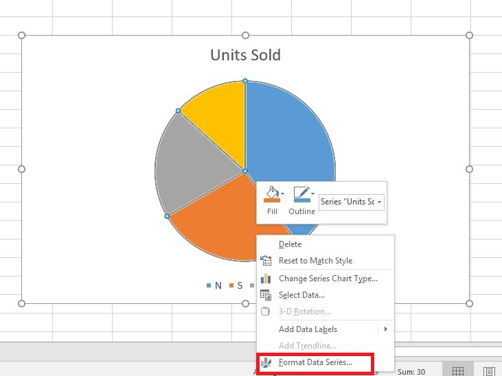
› excel-pie-chartExcel Pie Chart - How to Create & Customize? (Top 5 Types) The slices in an Excel Pie Chart appear according to the order of the data categories in the spreadsheet. We can rotate the Pie Chart for our analysis or to highlight any particular sector. Scenario 1: The procedure to Rotate a 2-D Pie Chart are as follows: Step 1: Right-click on the Pie Chart > select the “Format Data Series” option, as ...
3 Ways to Make Excel Chart Horizontal Categories Fit Better ...
Excel Pie Chart - How to Create & Customize? (Top 5 Types) The slices in an Excel Pie Chart appear according to the order of the data categories in the spreadsheet. We can rotate the Pie Chart for our analysis or to highlight any particular sector. Scenario 1: The procedure to Rotate a 2-D Pie Chart are as follows: Step 1: Right-click on the Pie Chart > select the “Format Data Series” option, as ...
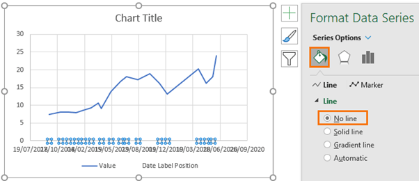
Label Specific Excel Chart Axis Dates • My Online Training Hub
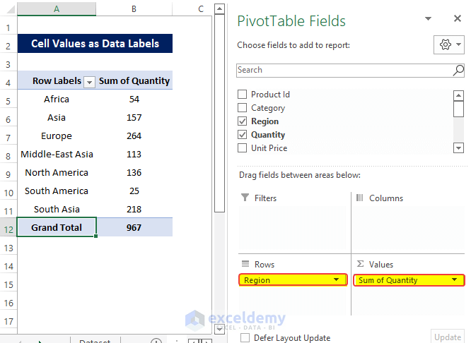
Data Labels in Excel Pivot Chart (Detailed Analysis) Aug 02, 2022 · Dragging the fields on the row will show them on the leftmost column as rows in the Pivot Table.; And adding them to the columns will place the values in the column in the Pivot Table.; You can change the value field settings, whether you want to show the Average value/Maximum/Minimum value etc.In the Value field area.; Next, we will discuss the Pivot …

How to Rotate Axis Labels in Excel (With Example) - Statology
Pivot Table Chart Axis Labels - Microsoft Community In the Pivot Table field well, click the "Full_Date" dropdown arrow and select Field Settings. Click the Number Format button. THIS is the dialog where pivot table formats for chart axes are determined. As I said, not very intuitive. Set the format to mmm-yy and it will change in both the pivot table and the pivot chart.
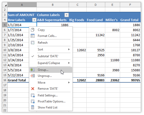
Group Items in a Pivot Table | DevExpress End-User Documentation
› data-labels-in-excel-pivot-chartData Labels in Excel Pivot Chart (Detailed Analysis) Aug 02, 2022 · 7 Suitable Examples with Data Labels in Excel Pivot Chart Considering All Factors. For the demonstration purpose, we are going to use the below dataset. This is hypothetical sales data of an imaginary organization, where we can see the ID of the products they sold so far, which Region they sold, their Type, Quantity, Cost of production, Ratings, Revenue, and Profit Margin.
Rotate Axis labels in Excel - Free Excel Tutorial
Home - Automate Excel Mar 07, 2022 · Chart Axis Text Instead of Numbers: Copy Chart Format: Create Chart with Date or Time: Curve Fitting: Export Chart as PDF: Add Axis Labels: Add Secondary Axis: Change Chart Series Name: Change Horizontal Axis Values: Create Chart in a Cell: Graph an Equation or Function: Overlay Two Graphs: Plot Multiple Lines: Rotate Pie Chart: Switch X and Y ...

Change axis labels in a chart
How to Make a Pareto Chart Using Pivot Tables in Excel Jul 18, 2022 · A useful guide to make a Pareto chart using Excel Pivot Tables. Download our practice book, modify data and exercise. ... Change Axis Alignment. The horizontal data labels are looking quite messy as the names are longer. ... Next, click on the Size & Properties icon and select Rotate All Text 270° from the Text direction dropdown box. Here’s ...
How to Customize Your Excel Pivot Chart Axes - dummies
How to I rotate data labels on a column chart so that they are ... To change the text direction, first of all, please double click on the data label and make sure the data are selected (with a box surrounded like following image). Then on your right panel, the Format Data Labels panel should be opened. Go to Text Options > Text Box > Text direction > Rotate
Change the display of chart axes
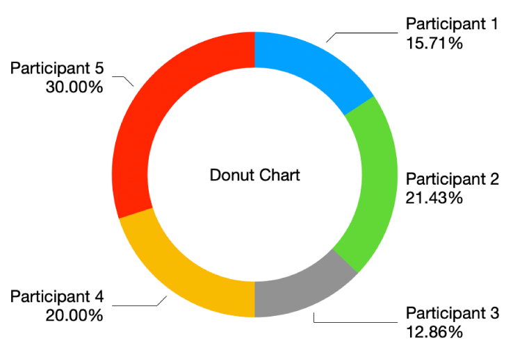
› how-to-show-percentage-inHow to Show Percentage in Pie Chart in Excel? - GeeksforGeeks Jun 29, 2021 · To add data labels, select the chart and then click on the “+” button in the top right corner of the pie chart and check the Data Labels button. Pie Chart It can be observed that the pie chart contains the value in the labels but our aim is to show the data labels in terms of percentage.
Rotate charts in Excel - spin bar, column, pie and line charts
Excel Chart: Multi-level Lables - Microsoft Q Excel Chart: Multi-level Lables. Hello experts! I have a bar chart that uses a multi-level category, similar to the example below. To save space in the Y axis labelling area, I'd like to have car manufacturers names on top of each bar while retaining the group names (=country) in the Y axis with a bar for each manufacturer.
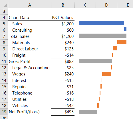
Excel Waterfall Charts • My Online Training Hub
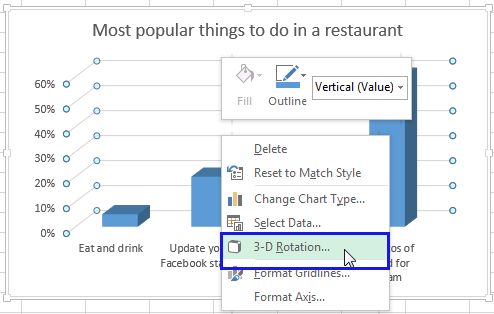
Rotate charts in Excel - spin bar, column, pie and line charts You can rotate your chart based on the Horizontal (Category) Axis. Right click on the Horizontal axis and select the Format Axis… item from the menu. You'll see the Format Axis pane. Just tick the checkbox next to Categories in reverse order to see you chart rotate to 180 degrees. Reverse the plotting order of values in a chart
3 Ways to Make Excel Chart Horizontal Categories Fit Better ...
How to Rotate Axis Labels in Excel (With Example) - Statology By default, Excel makes each label on the x-axis horizontal. However, this causes the labels to overlap in some areas and makes it difficult to read. Step 3: Rotate Axis Labels In this step, we will rotate the axis labels to make them easier to read. To do so, double click any of the values on the x-axis.

How to rotate text in axis category labels of Pivot Chart in Excel 2007? (3 Solutions!!)
Rotating axis text in pivot charts. | MrExcel Message Board Right Click on the Axis and choose Format Axis. Then find the Alignment area (depends on your version) Then Change Text Direction to Rotate All Text 270 degrees. Note that this will work only on the top level if you are utilizing the "Multi-Level Category Labels" feature of the chart. (i.e. if you have a grouped axis) Steve=True S Surveza

How to Rotate Axis Labels in Excel (With Example) - Statology
How to Show Percentage in Pie Chart in Excel? - GeeksforGeeks Jun 29, 2021 · The steps are as follows : Insert the data set in the form of a table as shown above in the cells of the Excel sheet. Select the data set and go to the Insert tab at the top of the Excel window.; Now, select Insert Doughnut or Pie chart.A drop-down will appear.
How to Rotate X Axis Labels in Chart - ExcelNotes
How to rotate axis labels in chart in Excel? - ExtendOffice Go to the chart and right click its axis labels you will rotate, and select the Format Axis from the context menu. 2. In the Format Axis pane in the right, click the Size & Properties button, click the Text direction box, and specify one direction from the drop down list. See screen shot below: The Best Office Productivity Tools
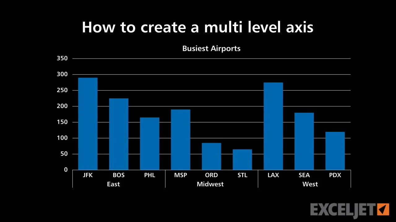
How to create a multi level axis
How to Rotate X Axis Labels in Chart - ExcelNotes
Change the look of chart text and labels in Numbers on Mac ...

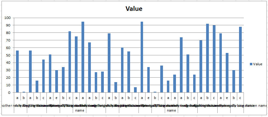
Stagger long axis labels and make one label stand out in an ...

Change axis labels in a chart
Data Labels in Excel Pivot Chart (Detailed Analysis) - ExcelDemy
Fixing Your Excel Chart When the Multi-Level Category Label ...

How To Rotate x-axis Text Labels in ggplot2 - Data Viz with ...
Excel Mac Pivot Charts - Can you switch rows and columns ...

r - Subgroup axes ggplot2 similar to Excel PivotChart - Stack ...
Label Specific Excel Chart Axis Dates • My Online Training Hub
How to Rotate X Axis Labels in Chart - ExcelNotes
Adjusting the Angle of Axis Labels (Microsoft Excel)

Bar charts with long category labels; Issue #428 November 27 ...
How to change/edit Pivot Chart's data source/axis/legends in ...

Pivot Charts in Excel Tutorial - Simon Sez IT

How to Rotate Data Labels in Excel (2 Simple Methods)
How to Rotate Pie Charts in Excel? - GeeksforGeeks

Pivot Charts in Excel Tutorial - Simon Sez IT
Pivot Chart Horizontal axis will not let me change both Axis ...
Where to Position the Y-Axis Label - PolicyViz
Text Labels on a Vertical Column Chart in Excel - Peltier Tech
Text Labels on a Vertical Column Chart in Excel - Peltier Tech

How to Add Axis Titles in a Microsoft Excel Chart
formatting - How to rotate text in axis category labels of ...
Post a Comment for "40 excel pivot chart rotate axis labels"