42 excel pivot table conditional formatting row labels
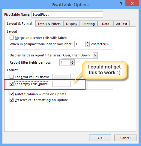
Design the layout and format of a PivotTable To change the layout of a PivotTable, you can change the PivotTable form and the way that fields, columns, rows, subtotals, empty cells and lines are displayed. To change the format of the PivotTable, you can apply a predefined style, banded rows, and conditional formatting. Windows Web Mac Changing the layout form of a PivotTable Excel 2010 Conditional Formatting Pivot Table Row Labels Home / Uncategorized / Excel 2010 Conditional Formatting Pivot Table Row Labels. Excel 2010 Conditional Formatting Pivot Table Row Labels. masuzi June 30, 2018 Uncategorized Leave a comment 14 Views. ... How To Apply Conditional Formatting Pivot Tables Excel Campus
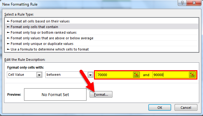
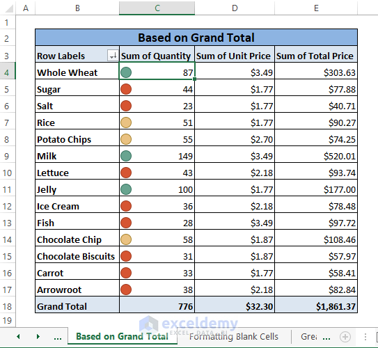
Excel Icon Sets conditional formatting: inbuilt and custom - Ablebits.com Select the range of cells where you want to apply the icons. Click Conditional Formatting > Icon Sets > More Rules. In the New Formatting Rule dialog box, select the desired icons. From the Type dropdown box, select Percentage, Number of Formula, and type the corresponding values in the Value boxes. Finally, click OK.
Excel pivot table conditional formatting row labels
Format Pivot Table Labels Based on Date Range Select all the dates in the Row Labels that you want to format. On the Ribbon, click the Home tab, and then in the Styles group, click Conditional Formatting. In the list of conditional formatting options, click Highlight Cells Rules, and then click A Date Occurring. Excel Pivot Table Conditional Formatting Row Labels All groups and messages ... ... Conditional Formatting on Pivot Table row labels As per my knowledge, in this case it does not matter what is the source of pivot as after getting the data in pivot, it's the pivot where the conditional formatting need to be applied, please upload a sample. thanks. Regards, DILIPandey DILIPandey +91 9810929744 dilipandey@gmail.com Register To Reply
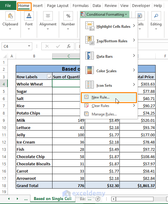
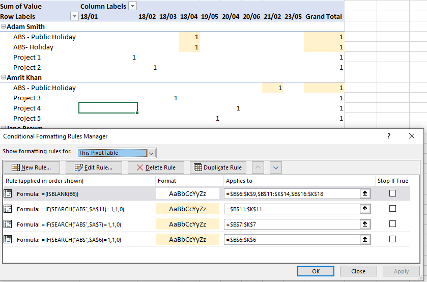
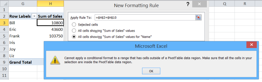
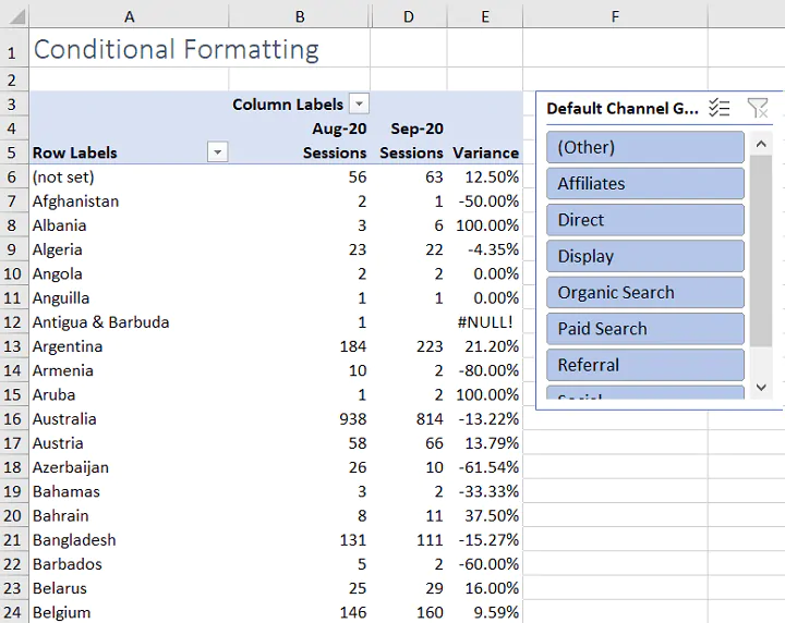
Excel pivot table conditional formatting row labels. How to Apply Conditional Formatting to Pivot Tables - Excel Campus So in this post I explain how to apply conditional formatting for pivot tables. 1. Select a cell in the Values area The first step is to select a cell in the Values area of the pivot table. If your pivot table has multiple fields in the Values area, select a cell for the field you want to apply the formatting to. 2. Apply Conditional Formatting Excel pivot table conditional formatting row labels jobs Search for jobs related to Excel pivot table conditional formatting row labels or hire on the world's largest freelancing marketplace with 21m+ jobs. It's free to sign up and bid on jobs. Re-Apply Pivot Table Conditional Formatting - yoursumbuddy This method relies on all the conditional formatting you want to re-apply being in that first row labels cell. In cases where the conditional formatting might not apply to the leftmost row label, I've still applied it to that column, but modified the condition to check which column it's in. This function can be modified and called from a ... Overwrite pivot table conditional format based on row label As far as I know, using the one rule in the Conditional formatting, we can only format the cells with one color if the condition is true and if the same condition is false, the formatting of the cell will be blank and if both conditions are true, the formatting of cell depends on the highest ranking/priority of the rules in Conditional formatting.
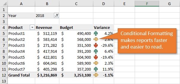
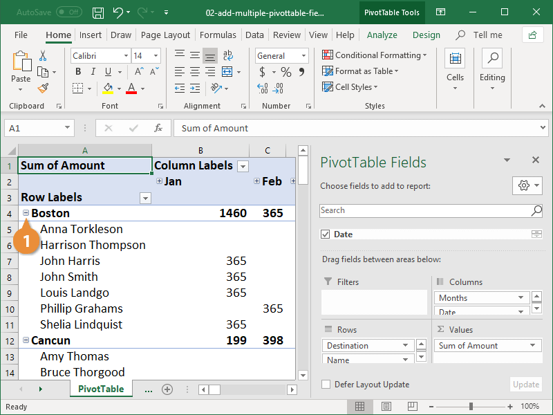
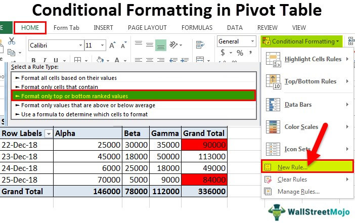
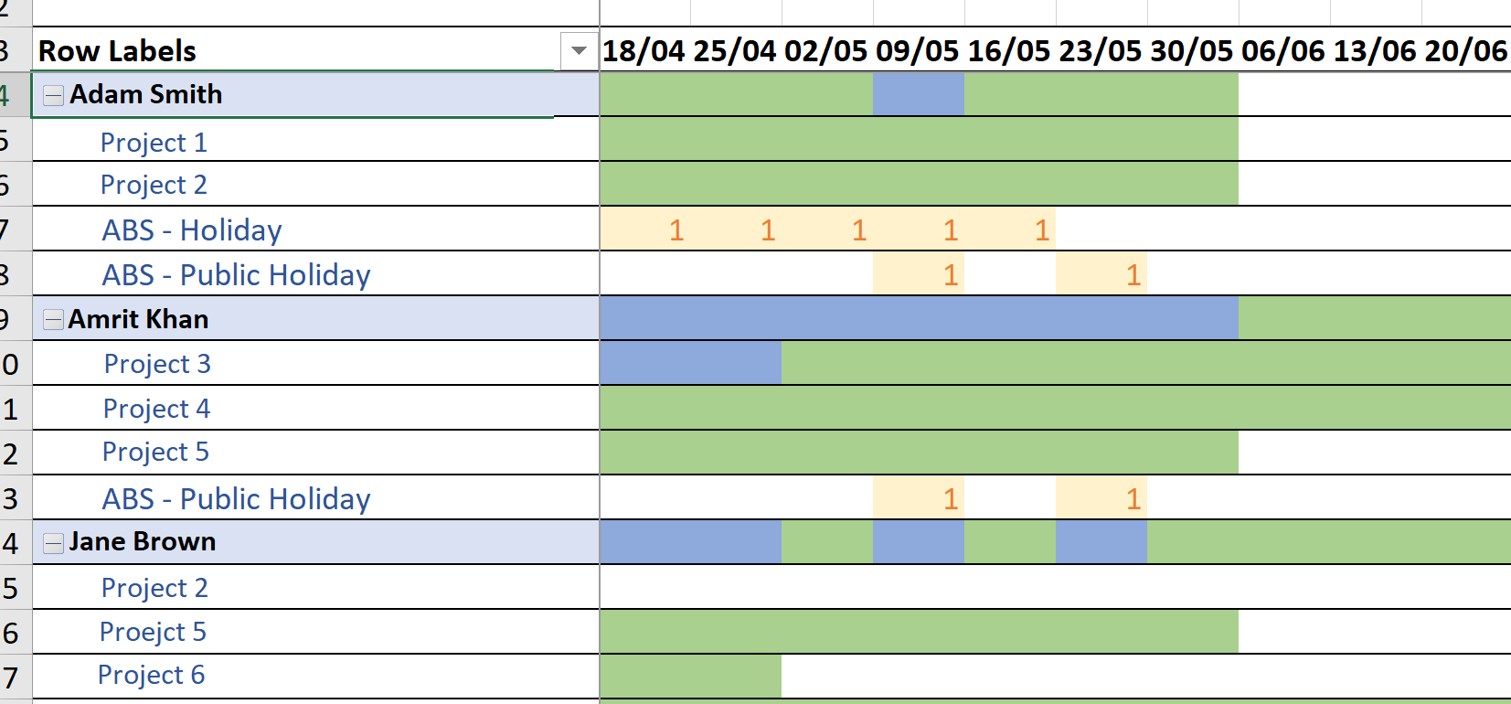
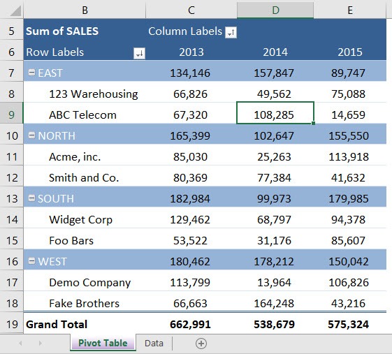
Conditional Formatting in Pivot Table - WallStreetMojo Currently, a pivot table is blank. Next, we need to bring in the values. Then, drag down the "Date" in the "Rows" Label, "Name" in the "Column," and "Sales" in "Values." As a result, the pivot table will look like the one below. To apply conditional formatting in the pivot table, first, we must select the column to format. Using column label as formatting condition in excel pivot table Using column label as formatting condition in excel pivot table Ask Question 0 I have pivot table in excel with sample data as attached. I now want to apply conditional formatting as red background where - data is between 10 to 25 AND - year is 2011 and 2012. =AND (C1="2011",OR (C2>10,C2<25)) Conditional Formatting of Pivot Tables - Excel TV Conditional Formatting of Pivot Tables. Xtreme Pivot Tables. Current Progress. Current Progress. Current Progress 0% Not ... Change SUM Views in Label Areas. Indent Rows in Compact Layouts. Change Layout of a Report Filter. ... New Excel 2013 Pivot Table Features. Cosmetic Changes. Recommended Pivot Tables. Distinct Count. Timeline Slicer. Pivot table drill down formatting - rlgo.atbeauty.info 2020. 7. 29. · Step 5: Gantt chart grid (right side portion) Now that our gantt chart is ready on the left, let's complete the grid. Start by calculating the earliest project start date using min formula =MIN (plan [Start date]) Place this formula in the grid top left cell, as shown below. Calculate remaining 89 dates by adding +1 working day.
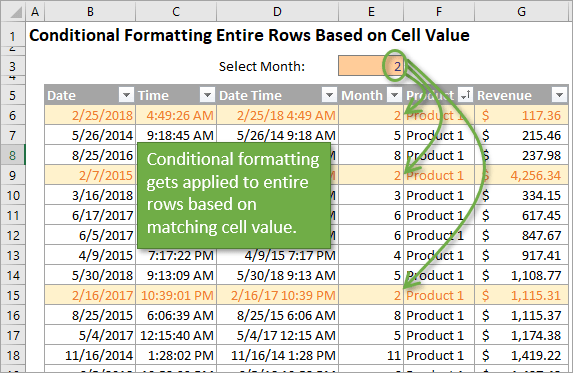
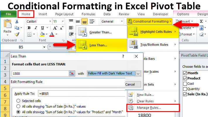
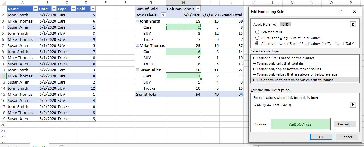
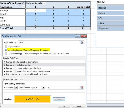
Pivot Table: Pivot table conditional formatting | Exceljet Select any cell in the data you wish to format and then choose "New rule" from the conditional formatting menu on the Home tab of the ribbon. At the top of the window, you will see setting for which cells to apply conditional formatting to. For the example shown, we want: "All cells showing sum of "sales values" for name and "date" Conditional Format Pivot Table Row | Chandoo.org Excel Forums - Become ... Select the entire row, and when you apply the conditional format, make the column reference absolute. So, say we want the entire row 2 to be formatted if cell in col B = 5. formula would be: =$B2=5 Pivot Table Conditional Formatting for Different Rows Items? Select Your Pivot Table and: Go to Conditional Formatting -> New Rule -> Choose All cells showing "duration" values for "Type and "Date Selection" under "Apply Rule To" section -> Use a Formula to Determine which cells to format and enter the following formula: =AND(A6="Cars",A6>3), You can create new rules for other two conditions as well: Excel Conditional Formatting in Pivot Table - EDUCBA Click on any cell in the pivot table > Go to the HOME tab > Click on Conditional Formatting option under Styles option > Click on Manage Rules option. It will open a Rules Manager dialog box. Click on the Edit Rule tab, as shown in the below screenshot. It will open the Editing Rule formatting window. Refer to the below screenshot.
Pivot Table Conditional Formatting Based on Another Column (8 ...
Pivot Table Row Label Date Formating | MrExcel Message Board Sep 25, 2014. #1. I have my pivot table set up. One of the row labels is a date field, however I cannot get it to stay in the date format I wish, it keeps defaulting to dd/mm/yyyy. The source column is set to format dd mmm yyyy. Every time I try something to change to date format in the pivot table, it defaults back again.
Overwrite pivot table conditional format based on row label ...
Conditional formatting of Row labels in pivot table I'm looking for a way to set up a condition in a pivot table to output or highlight any row labels that have more than 1 value listed under them. My pivot table has 2 fields listed under Rows. Each of these row labels should only expand with 1 value under them, i want to highlight or output any of the row labels that have more than 1 value listed under them.
How to Hide, Replace, Empty, Format (blank) values with an ...
Conditional Formatting on Pivot Table row labels As per my knowledge, in this case it does not matter what is the source of pivot as after getting the data in pivot, it's the pivot where the conditional formatting need to be applied, please upload a sample. thanks. Regards, DILIPandey DILIPandey +91 9810929744 dilipandey@gmail.com Register To Reply

Learn How to Apply Conditional Formatting in a Pivot Table ...
Excel Pivot Table Conditional Formatting Row Labels All groups and messages ... ...

Pivot Table Grouping, Ungrouping And Conditional Formatting
Format Pivot Table Labels Based on Date Range Select all the dates in the Row Labels that you want to format. On the Ribbon, click the Home tab, and then in the Styles group, click Conditional Formatting. In the list of conditional formatting options, click Highlight Cells Rules, and then click A Date Occurring.

How to Apply Conditional Formatting in Pivot Table? (with ...
How to Apply Conditional Formatting to Rows Based on Cell ...

Pivot Table Conditional Formatting
Conditional Formatting in Pivot Table (Example) | How To Apply?
How to Apply Conditional Formatting to Pivot Tables - Excel ...

Excel Conditional Formatting Entire Row Based on Cell Value

vba - Pivot Table with Conditional Formatting: Where did my ...
Pivot Table Conditional Formatting for Different Rows Items ...
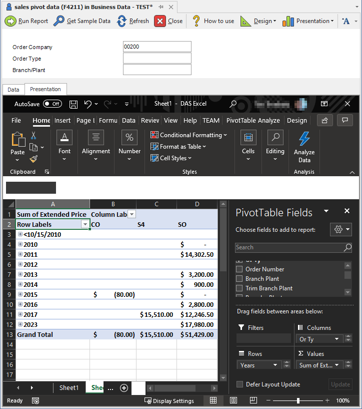
Excel Pivot Tables and Charts | ReportsNow DAS User Guide

How to apply conditional formatting to Pivot Tables

Pivot Table Grouping, Ungrouping And Conditional Formatting
Add Multiple Columns to a Pivot Table | CustomGuide
Highlight Cell Rules based on text labels | MyExcelOnline

Pivot Table: Pivot table conditional formatting | Exceljet
How to Apply Conditional Formatting in Pivot Table? (with ...

microsoft excel - In a pivot table, how to apply conditional ...
How to Apply Conditional Formatting in Pivot Table? (with ...
Overwrite pivot table conditional format based on row label ...
Maintaining Formatting when Refreshing PivotTables (Microsoft ...
How to Apply Conditional Formatting in Pivot Table? (with ...
Applying Conditional Formatting to a Pivot Table in Excel

pivot table row labels in separate columns 3 • AuditExcel.co.za

How to Replace Blank Cells with Zeros in Excel Pivot Tables

microsoft excel - In a pivot table, how to apply conditional ...
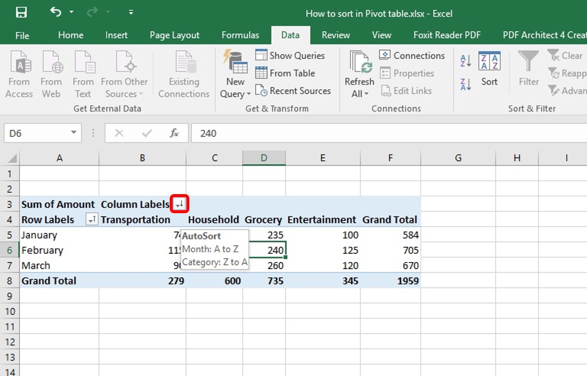
How to Sort Pivot Table | Custom Sort Pivot Table | A-Z, Z-A ...
Excel Pivot Tables - Sorting Data
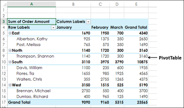
Pivot Table shows row labels instead of field name
Pivot Table Conditional Formatting | MyExcelOnline
Working with a Pivot Table that Has Conditional Formatting ...

EXCEL PRO TIP: Conditional PivotTable Formatting
How to Apply Conditional Formatting in Pivot Table? (with ...
Conditional Formatting in Excel - a Beginner's Guide

How to Apply Conditional Formatting to a Pivot Table in Your ...

Conditional format a Pivot Table with the wizards ...

microsoft excel - In a pivot table, how to apply conditional ...
Pivot Table Conditional Formatting Based on Another Column (8 ...
How to Apply Conditional Formatting to Pivot Tables - YouTube
Post a Comment for "42 excel pivot table conditional formatting row labels"