44 excel pie chart with lines to labels
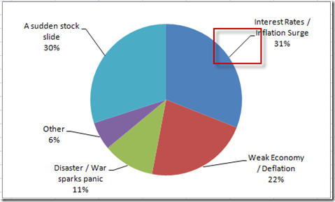
Display data point labels outside a pie chart in a paginated report ... Create a pie chart and display the data labels. Open the Properties pane. On the design surface, click on the pie itself to display the Category properties in the Properties pane. Expand the CustomAttributes node. A list of attributes for the pie chart is displayed. Set the PieLabelStyle property to Outside. Set the PieLineColor property to Black. How-to Add Label Leader Lines to an Excel Pie Chart 12 Jun 2013 — . It is that simple. Just make sure it is checked in the label options and then drag and drop an individual data label outside of the pie chart.
How to Create and Format a Pie Chart in Excel - Lifewire Jan 23, 2021 · To add data labels to a pie chart: Select the plot area of the pie chart. Right-click the chart. Select Add Data Labels . Select Add Data Labels. In this example, the sales for each cookie is added to the slices of the pie chart. Change Colors

Excel pie chart with lines to labels
How to Edit Pie Chart in Excel (All Possible Modifications) How to Edit Pie Chart in Excel 1. Change Chart Color 2. Change Background Color 3. Change Font of Pie Chart 4. Change Chart Border 5. Resize Pie Chart 6. Change Chart Title Position 7. Change Data Labels Position 8. Show Percentage on Data Labels 9. Change Pie Chart's Legend Position 10. Edit Pie Chart Using Switch Row/Column Button 11. Creating Pie Chart and Adding/Formatting Data Labels (Excel) Creating Pie Chart and Adding/Formatting Data Labels (Excel) Office: Display Data Labels in a Pie Chart - Tech-Recipes This will typically be done in Excel or PowerPoint, but any of the Office programs that supports charts will allow labels through this method. 1. Launch PowerPoint, and open the document that you want to edit. 2. If you have not inserted a chart yet, go to the Insert tab on the ribbon, and click the Chart option. 3.
Excel pie chart with lines to labels. Leader lines for Pie chart are appearing only when the data labels are ... I have a pie chart with data labels connected to leader lines. Though I have set the position of labels to 'Outside End', the leader lines are not appearing by default. It shows up only when I manually move the data labels. I dont have to move them far apart. Just a slight change in the position of labels helps. How to display leader lines in pie chart in Excel? To display leader lines in pie chart, you just need to check an option then drag the labels out. 1. Click at the chart, and right click to select Format Data Labels from context menu. 2. In the popping Format Data Labels dialog/pane, check Show Leader Lines in the Label Options section. See screenshot: 3. Excel 2010 pie chart data labels in case of "Best Fit" Based on my tested in Excel 2010, the data labels in the "Inside" or "Outside" is based on the data source. If the gap between the data is big, the data labels and leader lines is "outside" the chart. And if the gap between the data is small, the data labels and leader lines is "inside" the chart. Regards, George Zhao. TechNet Community Support. Directly Labeling in Excel - Evergreen Data There are two ways to do this. Way #1 Click on one line and you'll see how every data point shows up. If we add a label to every data points, our readers are going to mount a recall election. So carefully click again on just the last point on the right. Now right-click on that last point and select Add Data Label. THIS IS WHEN YOU BE CAREFUL.
Adding 2nd Data Label Series to Bar of Pie Chart If you use 2 sets of the same data in the chart you can create 2 pie/bar charts, with one appearing on the secondary axis. Make sure the settings for bar/pie formatting are the same. Add data labels to each series. Format one to show names the other values. Within the pie you may want to delete the name data labels. Attached Files Excel charts: add title, customize chart axis, legend and data labels To change what is displayed on the data labels in your chart, click the Chart Elements button > Data Labels > More options… This will bring up the Format Data Labels pane on the right of your worksheet. Switch to the Label Options tab, and select the option (s) you want under Label Contains: Pie chart leader lines in excel 2010 - Microsoft Community Replied on September 27, 2013. You the chart selector located in the Current Selection group of the Format contextual tab. Can you see 'Leader Lines 1' ? If yes select that item and use the Format selection button to display format dialog. Check Line Style is set to automatic, or alternative colour if that clashes with the chart area colour. If ... Excel custom pie chart labels - Microsoft Community Jul 08, 2019 · Excel custom pie chart labels. I want to use a pivot table to make a pie chart out of this. I want each of the pieces of the pie to contain the number of entries and between parentheses the percentage. So in the "Yes" piece, there should be '3 (33%)'. Actually, if I hover the pie chart in Excel, I get exactly the notation O want!
Pie Chart in Excel | How to Create Pie Chart - EDUCBA Step 1: Select the data to go to Insert, click on PIE, and select 3-D pie chart. Step 2: Now, it instantly creates the 3-D pie chart for you. Step 3: Right-click on the pie and select Add Data Labels. This will add all the values we are showing on the slices of the pie. Leader Lines in Excel Pie Charts - Microsoft Community Leader Lines in Excel Pie Charts. I've created pie charts in Excel. When I move the labels around I get leader lines that I do not want. I can delete them but if I save, close and then open the file, they come back. I can format the lines so that the color is white and they do not show. Dynamically Label Excel Chart Series Lines - My Online Training Hub Step 1: Duplicate the Series. The first trick here is that we have 2 series for each region; one for the line and one for the label, as you can see in the table below: Select columns B:J and insert a line chart (do not include column A). To modify the axis so the Year and Month labels are nested; right-click the chart > Select Data > Edit the ... Change the format of data labels in a chart To get there, after adding your data labels, select the data label to format, and then click Chart Elements > Data Labels > More Options. To go to the appropriate area, click one of the four icons ( Fill & Line, Effects, Size & Properties ( Layout & Properties in Outlook or Word), or Label Options) shown here.
How to Create and Label a Pie Chart in Excel 2013 : 8 Steps - Instructables
Advanced Excel - Leader Lines - Tutorials Point In earlier versions of Excel, only the pie charts had this functionality. Now, all the chart types with data label have this feature. Add a Leader Line Step 1 − Click on the data label. Step 2 − Drag it after you see the four-headed arrow. Step 3 − Move the data label. The Leader Line automatically adjusts and follows it. Format Leader Lines

How-to Add Label Leader Lines to an Excel Pie Chart - Excel Dashboard Templates
How to create a Titled and Labeled Excel Pie Chart with C# Creating a simple sample Excel Pie Chart, with labeled slices using C# and Excel Interop Pie in the Sky, not in your Eye This assumes you are using Excel Interop to work with Excel in a C# app. Creating a pie chart is as easy as generating some data for it, and adding the chart to a worksheet: C# Shrink Copy Code
How-to Add Label Leader Lines to an Excel Pie Chart - Excel Dashboard Templates
How to add leader lines to doughnut chart in Excel? Select data and click Insert > Other Charts > Doughnut. In Excel 2013, click Insert > Insert Pie or Doughnut Chart > Doughnut. 2. Select your original data again, and copy it by pressing Ctrl + C simultaneously, and then click at the inserted doughnut chart, then go to click Home > Paste > Paste Special. See screenshot: 3.

Excel 2013 Recommended Charts, Secondary Axis, Scatter & PivotCharts
How to Create Bar of Pie Chart in Excel? Step-by-Step From the Insert tab, select the drop down arrow next to 'Insert Pie or Doughnut Chart'. You should find this in the 'Charts' group. From the dropdown menu that appears, select the Bar of Pie option (under the 2-D Pie category). This will display a Bar of Pie chart that represents your selected data.
:max_bytes(150000):strip_icc()/Capture-5c84941446e0fb00013364fc.JPG)
33 How To Label Pie Chart In Excel - Labels Design Ideas 2020
Edit titles or data labels in a chart - support.microsoft.com The first click selects the data labels for the whole data series, and the second click selects the individual data label. Right-click the data label, and then click Format Data Label or Format Data Labels. Click Label Options if it's not selected, and then select the Reset Label Text check box. Top of Page

how to label pie chart in excel - Labels 2021
Add or remove data labels in a chart - support.microsoft.com To label one data point, after clicking the series, click that data point. In the upper right corner, next to the chart, click Add Chart Element > Data Labels. To change the location, click the arrow, and choose an option. If you want to show your data label inside a text bubble shape, click Data Callout.
Charts and Graphs Examples, Tutorials, and Samples for Microsoft Excel 2007
Put pie chart legend entries next to each slice - Microsoft Community Answer. Right-click on a freshly created chart that doesn't already have data labels. Choose Add Date Labels>Add Data Callouts. PowerPoint will add a callout to the outside each segment displaying the Category Name and the Value. Right click on a data label and choose Format Data Labels. Check Category Name to make it appear in the labels.

How to Create and Label a Pie Chart in Excel 2013 : 8 Steps - Instructables
How-to Add Label Leader Lines to an Excel Pie Chart - YouTube Step-by-Step Tutorial: how-to create label leader lines that connect pie labels that are outsi...
PIE chart labelling values with reference lines
Pie Charts how do you show Label and Value? | MrExcel Message Board Sub addlabels () ActiveSheet.ChartObjects ("Chart 3").Activate mycellpointer = 2 For Each p In ActiveChart.SeriesCollection (1).Points p.ApplyDataLabels Type:= _ xlDataLabelsShowLabel p.DataLabel.Select Selection.Text = "=Sheet1!R" & mycellpointer & "C6" mycellpointer = mycellpointer + 1 Next End Sub

33 How To Label A Pie Chart In Excel - Labels 2021
How to Make a Pie Chart in Excel (Only Guide You Need) From there select Charts and press on to Pie. You can also insert the pie chart directly from the insert option on top of the excel worksheet. Before inserting make sure to select the data you want to analyze. After this, you will see a pie chart is formed in your worksheet.
How-to Make a WSJ Excel Pie Chart with Labels Both Inside and Outside - Excel Dashboard Templates
How to Make a Pie Chart in Excel & Add Rich Data Labels to The Chart! A tennis coach at a hypothetical tennis clinic is evaluating the post-game performance of his top-seeded player. He wants to visually present the main types of errors the player made along with the unforced errors. Here we will combine this two errors in a pie chart. So let`s start the procedure. The source data is shown below:

CD: Pie of Pie Charts
excel - Positioning data labels in pie chart - Stack Overflow Sub tester () Dim se As Series Set se = Totalt.ChartObjects ("Inosa gule").Chart.SeriesCollection ("Grøn pil") se.ApplyDataLabels With se.DataLabels .NumberFormat = "0,0 %" With .Format.Fill .ForeColor.RGB = RGB (255, 255, 255) .Transparency = 0.15 End With .Position = xlLabelPositionCenter End With End Sub
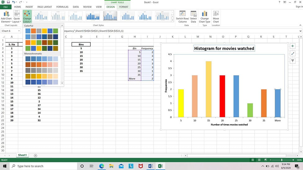
How to Create Histogram in Microsoft Excel? - My Chart Guide
How to Create Pie Charts in Excel (In Easy Steps) Click the + button on the right side of the chart and click the check box next to Data Labels. 10. Click the paintbrush icon on the right side of the chart and change the color scheme of the pie chart. Result: 11. Right click the pie chart and click Format Data Labels. 12. Check Category Name, uncheck Value, check Percentage and click Center.
Terrible Chart Tuesday - Leader Lines - Excel Dashboard Templates
Office: Display Data Labels in a Pie Chart - Tech-Recipes This will typically be done in Excel or PowerPoint, but any of the Office programs that supports charts will allow labels through this method. 1. Launch PowerPoint, and open the document that you want to edit. 2. If you have not inserted a chart yet, go to the Insert tab on the ribbon, and click the Chart option. 3.

How to Make a Pie Chart in Excel & Add Rich Data Labels to The Chart!
Creating Pie Chart and Adding/Formatting Data Labels (Excel) Creating Pie Chart and Adding/Formatting Data Labels (Excel)
How to Create a Pie Chart in Excel | Smartsheet
How to Edit Pie Chart in Excel (All Possible Modifications) How to Edit Pie Chart in Excel 1. Change Chart Color 2. Change Background Color 3. Change Font of Pie Chart 4. Change Chart Border 5. Resize Pie Chart 6. Change Chart Title Position 7. Change Data Labels Position 8. Show Percentage on Data Labels 9. Change Pie Chart's Legend Position 10. Edit Pie Chart Using Switch Row/Column Button 11.
33 How To Label Pie Chart In Excel - Labels Database 2020
Post a Comment for "44 excel pie chart with lines to labels"