40 excel pie chart add labels
How to Customize Your Excel Pivot Chart Data Labels - dummies The Data Labels command on the Design tab's Add Chart Element menu in Excel allows you to label data markers with values from your pivot table. When you click the command button, Excel displays a menu with commands corresponding to locations for the data labels: None, Center, Left, Right, Above, and Below. How to Edit Pie Chart in Excel (All Possible Modifications) 9. Change Pie Chart's Legend Position. Just like the chart title and data labels, you can also edit a pie chart in Excel by changing the position of the legend. Follow the simple steps below to do this. 👇. Steps: Firstly, click on the chart area. Following, click on the Chart Elements icon.
How to add Axis Labels (X & Y) in Excel & Google Sheets - Automate Excel This tutorial will explain how to add Axis Labels on the X & Y Axis in Excel and Google Sheets. How to Add Axis Labels (X&Y) in Excel. Graphs and charts in Excel are a great way to visualize a dataset in a way that is easy to understand. The user should be able to understand every aspect about what the visualization is trying to show right away.
Excel pie chart add labels
Pie of Pie Chart in Excel - Inserting, Customizing, Formatting To add the data labels:- Select the chart and click on + icon at the top right corner of chart. Mark the check box containing data labels. Formatting Data Labels Consequently, this is going to insert default data labels on the chart. Add / Move Data Labels in Charts - Excel & Google Sheets Adding Data Labels Click on the graph Select + Sign in the top right of the graph Check Data Labels Change Position of Data Labels Click on the arrow next to Data Labels to change the position of where the labels are in relation to the bar chart Final Graph with Data Labels How to add or move data labels in Excel chart? - ExtendOffice Add or move data labels in Excel chart 1. Click the chart to show the Chart Elements button . 2. Then click the Chart Elements, and check Data Labels, then you can click the arrow to choose an option about the data...
Excel pie chart add labels. Creating Pie Chart and Adding/Formatting Data Labels (Excel) Creating Pie Chart and Adding/Formatting Data Labels (Excel) How to Make a Pie Chart in Excel & Add Rich Data Labels to The Chart! 1) Select the data. 2) Go to Insert> Charts> click on the drop-down arrow next to Pie Chart and under 2-D Pie, select the Pie Chart, shown below. 3) Chang the chart title to Breakdown of Errors Made During the Match, by clicking on it and typing the new title. Microsoft Excel Tutorials: Add Data Labels to a Pie Chart To add the numbers from our E column (the viewing figures), left click on the pie chart itself to select it: The chart is selected when you can see all those blue circles surrounding it. Now right click the chart. You should get the following menu: From the menu, select Add Data Labels. New data labels will then appear on your chart: How to Create a Pie Chart in Excel | Smartsheet Enter data into Excel with the desired numerical values at the end of the list. Create a Pie of Pie chart. Double-click the primary chart to open the Format Data Series window. Click Options and adjust the value for Second plot contains the last to match the number of categories you want in the "other" category.
Pie Chart Examples | Types of Pie Charts in Excel with Examples It is similar to Pie of the pie chart, but the only difference is that instead of a sub pie chart, a sub bar chart will be created. With this, we have completed all the 2D charts, and now we will create a 3D Pie chart. 4. 3D PIE Chart. A 3D pie chart is similar to PIE, but it has depth in addition to length and breadth. How to Create Bar of Pie Chart in Excel? Step-by-Step Excel lets us add our own customizations to the Bar of Pie chart. For example, it lets us specify how we want the portions to get split between the pie and the stacked bar. It also lets us specify whether we want to display data labels, what data labels we want to be displayed as well as what formatting and styling we want to apply to the labels. Office: Display Data Labels in a Pie Chart - Tech-Recipes This will typically be done in Excel or PowerPoint, but any of the Office programs that supports charts will allow labels through this method. 1. Launch PowerPoint, and open the document that you want to edit. 2. If you have not inserted a chart yet, go to the Insert tab on the ribbon, and click the Chart option. 3. How-to Add Label Leader Lines to an Excel Pie Chart - YouTube Step-by-Step Tutorial: how-to create label leader lines that connect pie labels that are outsi...
How to display leader lines in pie chart in Excel? - ExtendOffice To display leader lines in pie chart, you just need to check an option then drag the labels out. 1. Click at the chart, and right click to select Format Data Labels from context menu. 2. In the popping Format Data Labels dialog/pane, check Show Leader Lines in the Label Options section. See screenshot: 3. How to Create Pie Charts in Excel: The Ultimate Guide How to Add Labels to a Pie Chart in Excel. Adding labels to a pie chart is a great way to provide additional information about the data in the chart. To add click format data labels, select the pie chart and then go to the ribbon and click on the Add Data Labels button. This will add data labels for each pie chart slice that show the value of ... Adding data labels to a pie chart - Excel General - OzGrid With ActiveChart.SeriesCollection(1) ' HasDataLabels is a valid property .HasDataLabels = True ' XL2000 pie chart .ApplyDataLabels Type:=xlDataLabelsShowPercent _ , AutoText:=True, LegendKey:=False, HasLeaderLines:=True ' XL2003 pie chart ' .ApplyDataLabels AutoText:=True, LegendKey:= _ ' False, HasLeaderLines:=True, ShowSeriesName:=True, 'ShowCategoryName:=True _ ' , ShowValue:=True, ShowPercentage:=True, 'ShowBubbleSize:=False, _ ' Separator:=", " With .DataLabels .Font.Bold = True With ... Add data labels and callouts to charts in Excel 365 - EasyTweaks.com Step #1: After generating the chart in Excel, right-click anywhere within the chart and select Add labels . Note that you can also select the very handy option of Adding data Callouts.
microsoft excel - How to make a Pie radar chart - Super User
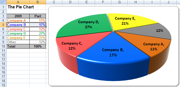
How to Show Percentage in Pie Chart in Excel? - GeeksforGeeks 29-06-2021 · Select a 2-D pie chart from the drop-down. A pie chart will be built. Select -> Insert -> Doughnut or Pie Chart -> 2-D Pie. Initially, the pie chart will not have any data labels in it. To add data labels, select the chart and then click on the “+” button in the top right corner of the pie chart and check the Data Labels button.

Microsoft Excel Tutorials: Add Data Labels to a Pie Chart
How To Make A Pie Chart In Excel: In Just 2 Minutes [2022] How To Make A Pie Chart In Excel. In Just 2 Minutes! Written by co-founder Kasper Langmann, Microsoft Office Specialist. The pie chart is one of the most commonly used charts in Excel. Why? Because it’s so useful 🙂. Pie charts can show a lot of information in a small amount of space. They primarily show how different values add up to a whole.
How to Create a Pie Chart in Excel (with Pictures) | eHow
c# - Add data labels to excel pie chart - Stack Overflow I am drawing a pie chart with some data: private void DrawFractionChart(Excel.Worksheet activeSheet, Excel.ChartObjects xlCharts, Excel.Range xRange, Excel.Range yRange) { Excel.ChartObject ... Adding labels to markers in Excel from a column in C#. Related. 963.NET String.Format() to add commas in thousands place for a number.

Creating Pie Chart and Adding/Formatting Data Labels (Excel) - YouTube
Pie Chart in Excel - Inserting, Formatting, Filters, Data Labels To add Data Labels, Click on the + icon on the top right corner of the chart and mark the data label checkbox. You can also unmark the legends as we will add legend keys in the data labels. We can also format these data labels to show both percentage contribution and legend:- Right click on the Data Labels on the chart.
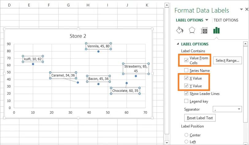
Add Custom Labels to x-y Scatter plot in Excel - DataScience Made Simple
charts - Excel, giving data labels to only the top/bottom X% values ... Here is what you can do, in stages: 1) Create a data set next to your original series column with only the values you want labels for (again, this can be formula driven to only select the top / bottom n values). See column D below. 2) Add this data series to the chart and show the data labels. 3) Set the line color to No Line, so that it does ...
Excel 3-D Pie Charts
Pie Chart in Excel | How to Create Pie Chart - EDUCBA Example #2 - 3D Pie Chart in Excel Step 1: . Select the data to go to Insert, click on PIE, and select 3-D pie chart. Step 2: . Now, it instantly creates the 3-D pie chart for you. Step 3: . Right-click on the pie and select Add Data Labels. This will add all the values we are showing on the ...

Excel Dashboard Templates How-to Add Label Leader Lines to an Excel Pie Chart - Excel Dashboard ...
How to Insert Axis Labels In An Excel Chart | Excelchat We will go to Chart Design and select Add Chart Element Figure 6 - Insert axis labels in Excel In the drop-down menu, we will click on Axis Titles, and subsequently, select Primary vertical Figure 7 - Edit vertical axis labels in Excel Now, we can enter the name we want for the primary vertical axis label.

How to Create a Pie Chart in Excel | Smartsheet
How to Use Cell Values for Excel Chart Labels Select the chart, choose the "Chart Elements" option, click the "Data Labels" arrow, and then "More Options.". Uncheck the "Value" box and check the "Value From Cells" box. Select cells C2:C6 to use for the data label range and then click the "OK" button. The values from these cells are now used for the chart data labels.
Post a Comment for "40 excel pie chart add labels"